
The first example is an experimental data set generated by Dr. Bill Lawless [4] a psychologist at Paine College in Augusta Georgia. The objective was to generate a data set that would allow a psychologist to select 5 AirForce pilots out of 20 that would constitute the best possible of all combinations for a particular mission. The selection is made by testing all 20 prospective pilots' under three test conditions over a ten day period. The selection is made by monitoring pilots choices to the test conditions. Hence, choice, C, becomes a function of pilot's personality, p, test condition, TC, and time, t.
Function: C = C( p, TC, t ) (2)
Following the previously defined visual data compression method, we avoid drawing the family-of-curves figures and immediately draw the final compressed format shown in the schematic figure, Fig. 7, shown below.

Figure 7. Compressed psychological experimental data
Because this is an experimental data set, we want to avoid eliminating data until we can make a comparison. From our recently defined visual method we can indeed postpone eliminating any data until we view it all at once. Hence our conclusions are based on observing all the data first. With this method the observer can also find unexpected trends in the data, which is similar to the analytic example, Fig. 2. These two tasks: viewing all data and looking for trends, could only be accomplished by a method that does not require data reduction or simplification of data a priori.
There are several interesting aspects of this data set that are quite different from the previous analytic data set. Except for time there is no particular ordering of data along the personality or test condition axes: parameters along axes do not have to be continuous. Stretching data along the TC axis allows the viewer to compare results. For null test results we can simply use transparency similar to that used in Fig. 3 where we are not required to use a particular color. Indeed for the null data we are not cognitively required to process "see" data as a particular color and then required to make a mental effort to disregard that color. Recall Tufte's examples on "chart junk" [1]. A well designed interface is not seen. In this example the viewer is not required to view purple, hence, the viewer's efforts focus only on relevant data. This part of the data interface literally becomes transparent.
Results are shown in Fig. 8 where the following interactive investigative process is summarized. In the bottom plane of Fig. 8a we observe the initial distribution of competitive and cooperative choices. If we move the bottom plane up in time we observe how each personality in a comparative format changed their choice with time. A revealing observation in one plane often directs the observer to select and move another plane perpendicular (orthogonal) to the first. For example in Fig. 8a we move a vertical plane over the most competitive personality and observe that this individual became cooperative in Fig. 8b. This raises the question whether similar trends can be observed for other personalities. Hence, we move a third orthogonal plane over all competitive responses and find one individual who maintains a competitive response in Fig. 8c. A fourth plane is moved to that region in Fig. 8c and shows that this individual is competitive only for that one test condition, Fig. 8d.

Figure 8. Simple example of an interactive session.
To make the same observations and interact with the data in a family-of-curves format would be impossible. We recall in Tufte's example of "from tables to graphs" that accuracy in data is not a requirement when observing and comparing functions. The desired function can be more accurately selected from the graphs than from the tables. Accurate data should not be confused with making an accurate selection from what could be a confusing array of functions. From studying this experimental data set we conclude that the observer can make a quick decision with high confidence because all measured data were observed in a comparative-interactive-compressed format. In general this method should work well when massive data sets are constantly changing and decisions are based on the existence of functions embedded within this data.
The second example is an analytic function but unlike the first analytic function, eqn. (1), there is a physical basis for this function, hence, there is an opportunity to relate our function to the geometry and physics of this particular problem. This function is given below where the strain, Ezz, is a function of the crack radius, rc, fiber volume fraction, Vf, and elastic property ratio, R, taken from a report [5] written by Carman, Lesko, and Reifsnider.
 (3)
(3)
The function given above is derived from the boundary value problem shown below in Fig. 9, where the unidirectional fiber-reinforced composite sustains a crack in the center fiber of a composite subject to a prescribed remote strain and the crack grows towards the adjacent fibers. The strains at the interface of the adjacent fibers are identical due to symmetry and these strains should increase with increasing crack growth. The effect of increasing fiber volume fraction and elastic property ratio on the interface strain is less obvious, but the physics would suggest an increasing strain with increasing fiber volume fraction and elastic property ratio. As before with eqn. (1), trends can not be deduced from eqn. (3) because the complexity of the analytic function does not suggest a possible trend, "it goes like". Here our objective is to better understand the relationship between interfacial strains over a range of parameters that can be physically controlled during fabrication of this composite material system. Hence like the previous experimental data set we are also interested in choosing from a range of possible parameters where this selection process results in a well designed composite material system. Again this selection process can best be accomplished using the compressed-interactive-comparative format.
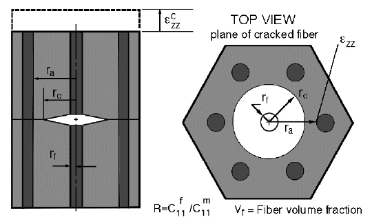
Figure 9. Physical parameters defined for fiber fracture model.
Again we avoid using the family -of-curves format and immediately construct the function in the comparative-interactive-compressed format as shown in Fig. 10. Before moving any planes, we observe the highest strain appears in the lower left corner where R=1, rc = ra, and Vf.
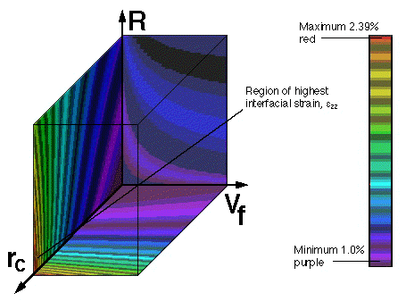
Figure 10. Interfacial strain relationship with material parameters.
As in the previous examples the horizontal rc - Vf plane is the initial plane of interest but as shown in Fig. 11 movement of this plane reveals little new information. In Fig. 12, the strain variations observed in the rc - R plane reveal a minimum strain over a large range of fiber volume fractions. But in Fig. 13 we observe a minimum strain only for the larger crack lengths. In these figures we observe that for a given crack length we can choose an optimum fiber volume fraction and elastic property ratio that will minimize the interfacial strain at the unbroken neighboring fibers. Note that both the fiber volume fraction and elastic property ratio can be controlled by the material engineer who is designing this material system. Hence we can use this visual method to optimize the fabrication of a material system for a given property: in this example we have minimized the strain to failure of adjacent fibers. Of course the same result could have been obtained by using a variational analytic method, but only if the function is differentiable. In some cases a numerical method is appropriate when an analytic approach is impossible. In either case it may be desirable to first observe in a comparative format which parameters are the best candidates for optimization. Again we find that by using a visual comparative method first, we can more efficiently use numerical, analytical or experimental methods which are better at providing quantitative information. Hence visual methods complement existing methods.
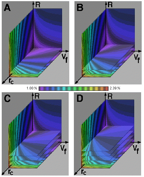
Figure 11. Variation in interfacial strain in the rc - Vf plane at various values for R.
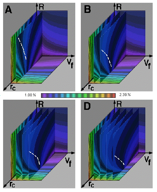
Figure 12. Variation in interfacial strain in the rc - R plane at various values for Vf.
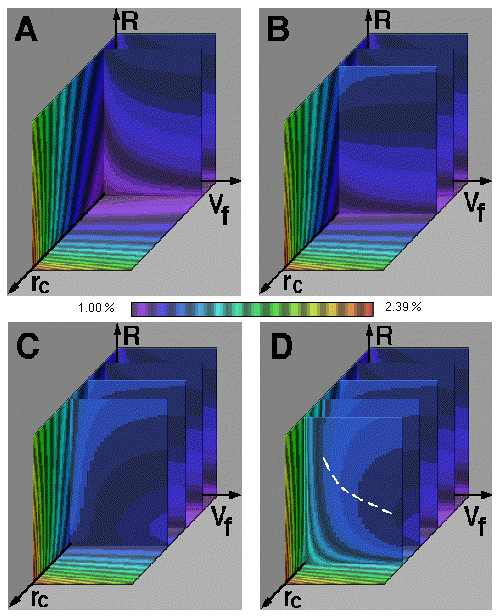
Figure 13. Variation in interfacial strain in the Vf - R plane at various values for rc.
 Click image to
return to Visualization home page.