Keywords: computerized tomography, serial algorithm, parallel algorithms, Matlab, Paragon, CM-5.
Computer Tomography(CT) is used in several applications --- medicine, non-destructive testing/evaluation, astronomy and others to look inside objects and analyze internal structures. However, the problem in general is computationally very intensive. The large computational requirement has led to large times for CT reconstruction. This has hindered the use of CT in many applications where CT image data is required in real time. Parallel processing is one of the techniques available which can reduce the reconstruction time very significantly. In this project, we describe a parallel implementation of the filtered back projection algorithm for finding 2D cross sectional images. The results show that parallel processing is very viable for CT reconstruction and results in significant run time savings. We describe an implementation on two different machines: the Intel Paragon and the Connection Machine. For comparison, the filtered back projection algorithm was first programmed as a serial algorithm using Matlab software on a Sun Sparc 10. It has been found that while the serial program in Matlab takes approximately 12 minutes for a reconstruction, the same data can be parallelized on the Intel Paragon in about 2.2 secs and on the CM5 in about 3 secs.
Authors acknowledge NASA Langley Research Center (NASA grant number NAS1-1847 task #49), NCSA (Grant Number DMR93002N) for access to the CM-5, and Dr. Layne Watson for access to the Virginia Tech's HPCC: Paragon.
Computer Tomography(CT) refers to the cross-sectional imaging of an object from its projection data. The mathematical basis for CT was first discovered by Radon in 1917 [1]. However, it was not until 1972 that the first CT scanner was invented,for which G.N. Hounsfield and Alan McCormack received the Nobel Prize [2]. Since then, many advances have been made in scanner technology as well as in the algorithms used for CT reconstruction. Today CT scanners are used extensively in many applications (medicine, astronomy and non-destructive testing) to carry out three dimensional volume visualization of objects [3,4].

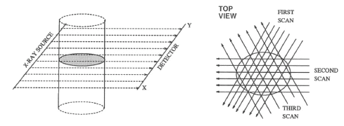
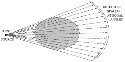
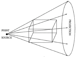
Fundamentally, tomography deals with reconstruction of an object from its projections. The technique of tomography consists of passing a series of rays (in parallel, fan or cone formation) through an object, and measuring the attenuation in these rays by placing a series of detectors on the receiving side of the object. These measurements are called projections. This data is collected at various angles from 0 to 360 degrees. Any of several algorithms available can then be used to reconstruct its 2D cross-sectional image from its projections. The property that is actually computed is the linear attenuation coefficient of that object, at various points in the object's cross-section. If this process is repeated at various heights along the object, we obtain several 2D cross-sectional images, which can then be stacked one on the top of another to get internal 3D volume vizualization of the object. There are many methods of collecting the projection data. The first is called "parallel projection" and is illustrated in fig. (1.1). There are other methods for collecting the projection data such as fan beam, and conee beam projections as shown in figs. (1.2) and (1.3). In this paper, we considered parallel beam projection data only. The algorithms used for parallel beam reconstruction can also be used for fan beam projections as well with some changes.
Serial implementation of the filtered back projection algorithm is time consuming and does not give the images in real time. We have parallelized the serial algorithm to achieve a very significant speed up as compared to the serial algorithm (minutes vs. a few seconds). The method adopted in the parallelization has been row-wise distribution of the data - and then carrying out the same instructions on the different data. The row-wise distribution results basically in the distribution of the projection data for different angles on different processors.
This paper describes the implementation of the filtered back-projection algorithm on a multiprocessor Intel Paragon and the Connection Machine (CM5). Implementation of the algorithm on these machines has led to new algorithms for parallel implementation, and these are described in this report. It is seen that parallel processing leads to significant improvements in the computing time requirements.
The mathematical basis for tomography was originally developed by Radon in 1917 [1]. There was dormancy in the fielduntil the invention of the first CT scanner in 1972 by G.N. Hounsfield and Alan McCormack [2], considered to be a major breakthrough in the field of Computed Tomography. The filtered back-projection algorithm was invented by Bracewell and Riddle [6], and later independently with additional insights by Ramanchandran and Lakshminarayanan [3,5] who are also responsible for the convolution back-projection algorithm. This is the algorithm now used by almost all commercially available CT scanners [3]. The filtered back-projection algorithm for fan beam data was developed by Lakshminarayanan [7]. Several researchers have proposed algebraic techniques for reconstruction: Gordon [8,9], Herman [10, 11] and Budinger [12]. Wernecke and D'Addario [13] proposed a maximum entropy method for reconstruction. It was shown by Shepp and Logan [14] that the filtered back-projection method is much superior to other methods (especially the algebraic methods) in 1974.
Several methods for improving the speed of the algorithms have been proposed.These can broadly be classified in three categories: (a) Improvements in the algorithms, (b) Improvements in the hardware used for computing the reconstructions, and (c) Parallel processing techniques. Under category (a) we have the work of Tanaka [15], Kenue [16], Wang [17], Dreike [18] and several others. Peters [20] developed the STRETCH algorithm which used precomputed look-up tables for interpolation.
Improvements in hardware, and the use of dedicated hardware has been suggested by several workers: Thompson et. al. [20] implemented special hardware to implement the STRETCH algorithm. Hartz et. al. [21] have implemented a special hardware for carrying out backprojection on an event by event basis with two microseconds per event in positron CT. More recently, Agi [22] have come up with the VLSI implementation of a dedicated microprocessor for carrying out forward and backward Radon transform. They make extensive use of pipelining to achieve faster processing. It has been shown that 64 of these Application Specific Integrated Circuits (ASIC's) will backproject 512x512 pixel raster-scan image from filtered CT data in 70 ms [22]. Although ASIC's have advantages in many applications, in this case since multiprocessing is required, it becomes less practical to use an ASIC as they offer less flexibility to the user.
Parallel implementation of CT algorithms became important when it became necessary to reconstruct 3D images in real time [23]. Studies have indicated that parallel implementation is the only way to implement 3D reconstruction algorithms in real time [23,24,25]. Jones et. al. [26] proposed a scheme for parallelizing the Expectation Maximization algorithm. Pixels are circulated through the processing elements(PE's), each of which backprojects one view of the projection data. Lacer et. al. [27] have proposed a multiprocessor scheme for the Maximum Liklehood Estimator(MLE) based algorithm. All the matrices are partitioned into disjoint segments which are stored in different sections of memory. Each PE has direct access to one of these memory sections --- and the other PE's can access the same through a cross-bar switch. The use of a cross-bar switch limits the maximum number of processors which can be used, as the cost of switching increases very fast for large number of processors. Both the above parallel implementations discussed are for iterative type of algorithms. Chen et. al. [23] have implemented the filtered back-projection algorithm on an Intel iPSC/2 --- a hypercube system with 32 nodes. Convolution was done in the spatial domain (instead of the frequency domain) to reduce the memory requirements (as zero padding of data has to be done to reduce errors). The projection data as well as the response function were distributed to all the nodes; convolution was done in parallel by carrying out all the multiplications on different processors in parallel. Then the intermediate results are sent to a designated node(PE) where the additions were performed. In the back-projection stage, they used the 3D incremental incremental algorithm developed by Cho et. al. [24]. Heree back-projection is performed on a beam by beam basis by each PE, and the final image is collected by a designated processor. Broadcasting and integration (of messages) can be done in O(logN) steps. But a major disadvantage of their method seems to be that a lot time is spent in interprocessor communication, as even the convolution is done in parallel. Also, it seems that carrying out convolution in the spatial domain (and not in the frequency domain where fast algorithms like the FFT can be used) is also a waste of computing power. Atkins et. al. [28] have implemented the STRETCH algorithm for use in 3D PET (positron emission tomography). The transputers (T800's) were connected in a tree type of arrangment with one node working as a master and the others as workers. They used the same transputers for speeding up the data acquisition, image reconstruction and display [28, 29]. They have estimated that 3D images could be reconstructed in about 10 minutes using about 200 nodes (T800's) in a tree type of interconnection. Barresi et al. have also implemented the 3D filtered back-projection algorithm on Transputers(T800) using the OCCAM programming language [25]. They tested their algorithms on a 5 transputer network, and they also used parallel FFT algorithms for finding the FFT. They have reported a reconstruction frequency of 700Hz with 5 T800 Transputers.
In this project, we have implemented the filtered back-projection algorithm for 2D on two different parallel platforms: a 28 node Intel Paragon with the nodes connected as a mesh, and a CM5 (Connection Machine). The Paragon implementation is fully complete with message passing controlled by the parallel algorithm. Although both the implementations have been done in high level languages (using the parallel constructs provided by the language compilers on those machine), the CM5 software is parallelized by the Connection Machine compilers, and so we do not have explicit control on the message passing (unlike the Intel Paragon). On the Intel Paragon we have implemented an explicit message passing algorithm using the message passing constructs provided on the machine. The parallel times were compared with the serial algorithm in Matlab.
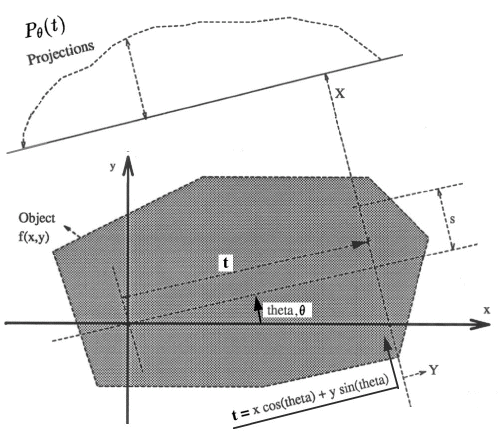
Let x,y represent the coordinates inside the object (fig. 2.1), and f(x,y) the density (attenuation coefficient) in rectangular co-ordinates of the object under consideration at the cross-section at which the imaging has to be done. Let eqn 2.1 represent the projection of the object at distance, t, from the center. The equation of the line AB is = x cos(theta)+y sin(theta), where we use "theta" (rotation angle) in place of the greek symbol. Then, the projections are defined as [3]:

It has been shown [3] that the above equation can be written using a delta function as:

This function is known as the Radon transform of f(x,y) [3]. A set of these functions for constant angle are the projections of the object at the cross-section where the rays are being passed. When the angle "theta" is held constant throughout a projection, we get parallel projection data. If a point source is used, we get fan beam projection data. The name fan beam results from the fact that the line integrals are measured along fans [3,4].

where u,v are measured in cycles/unit length. From the definition of the 1D fourier transform, we can find the Fourier Transform of the projection data at any angle as:

where, w is the in radians/unit length.
We define a new co-ordinate system (t,s) defined by the rotation of the (x,y) system by the angle of rotation such that

In the (t,s) co-ordinate system, a projection would then be defined as

From eqns. (2.4) and (2.5), we can say that

This can be transformed into the (x,y) co-ordinate system using the result of eqn. (2.5) to get the following result:

The right hand side of eqn.(2.8) represents the two-dimensional Fourier transform of the density f(x,y) and left hand side is the 1D Fourier transform of the projections. Therefore, taking the 1D Fourier transform of the projections of an object at an angle "theta" is equivalent to obtaining the two dimensional Fourier transform of the density f(x,y) along the line "t" inclined at an angle "theta" Therefore if we take these projections at many angles, then we can get this 2D Fourier transform of the projections at many such lines inclined at various angles. If the number of angles is large enough, we will get many lines of 2D Fourier transforms of the object. If we now find the inverse fourier transform of all these lines, we get the object's densities f(x,y) for all (x,y) in the object's cross-section. That is,

represents the back projection along the line t,
where,

This is the Fourier Slice Theorem, and in essence provides a justification for using the Fourier theory in CT algorithms. A more detailed proof can be found in [3], [5] and [6].
Proof of the filtered back projection algorithm follows from eqn. (2.10) [3,5,7,4]. The following proof is due to Kak and Slaney [3]. If the co-ordinate system in the frequency domain (u,v) which is rectangular is changed to the polar co-ordinate system, we have to make the following substitutions:

where, w = radius and the theta symbol = angle in radians and the differentials change as

We can split the above integral by considering "theta" from 0 radians to "pi" radians, and then from "pi" radians to 2 "pi" radians. We then get,

But it is known from Fourier theory that [3,5,7]

Therefore simplifying eqn. (2.15) we get:

From (2.4) and (2.7), we can say that in this case, F(w, "theta") inside the integral is the same as S(w) of eqn. (2.7). Therefore,

In the Eqn. (2.18) above, the terms inside the square brackets (the operation indicated by the inner integral) represents a filtering operation and evaluate the filtered projections, and the operation being performed by the outer integral evaluate the back-projections, which basically represents a smearing of the filtered projections back on to the object and then finding the mean over all the angles.
The filtered back projection algorithm can therefore be thought of as a three step process:
1. Finding the Fourier Transform (FT) in 1D of the projections.
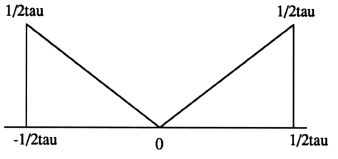
2. Finding the filtered projections. This essentially means multiplying the results of step 1. with a response function whose function looks as shown in fig.(2.2) in the frequency domain, and then finding the inverse Fourier Transform (IFFT) . This step is essentially the same as carrying out convolution in the time domain. It can be represented mathematically as

3. Finding the back projections. This step is the smearing of the filtered projections back on to the object, and is mathematically represented by

These three steps represent the filtered back projection algorithm. In the discrete domain, the algorithm changes only slightly. The important steps are outlined below:
1. Find the 1D FT of the projections for each angle.
2. Multiply the result of step 1. above with the response function in the frequency domain (equivalent to convolving with the response function in the time domain). In the actual simulations, the response function is simply a ramp with 45 degree slope and with the same length as the finalreconstructed image. (In the function shown in fig. (2.2), the vertical magniture represents the distance between the rays).
3. Find the IFFT of the results in step 2. This gives us the filtered projections in the discrete domain and correspond to Q(n), where the Q's are taken at the various angles at which the projections were taken, and "n" is the ray number at which the line projection was taken.
4. Back-project. The integral of the continuous time system now becomes a summation, and we get

It should be noted here that (x,y) are chosen by the program while back projecting. So the value of x cos (theta) + y sin (theta) may not correspond exactly to a value of "n" for the filtered projections which may have been calculated in the previous step. Therefore interpolation has to be done, and usually linear interpolation is quite sufficient [3]. It may be noted that in terms of computational time, this step consumes the maximum time (about 80%). Many authors have proposed different strategies for coping with this computational demand. One popular method is to find the filtered projections for a very large number of points by heavily zero-padding the original data. Then, while back-projecting, the nearest or closest point can be selected. In our implementation, we carry out the linear interpolation to get realisticestimates of the speed of the linear and parallel algorithms. We however, zero-pad the data to four times its length to remove the dishing and dc artifacts from the final images. These artifacts are a result of the finite number of frequencies which can be represented in the discrete Fourier transform(DFT) [3]; it is usually recommended to zero-pad to double the length of the vectors to reduce dishing and dc artifacts [3,30]. Zero-padding gives a better resolution in the frequency domain and the Fast Fourier Transform (FFT) algorithm normally used in computing the DFT is more accurate if larger point sizes are used [3,30].
We now clarify some CT terminology. A bin is a detector where a ray was received. The term mid bin refers to the point where the ray should have been received if the ray corresponding to a particular x and y points had a detector. However, detectors (bins) are just spaced at equal intervals, and so all the points inside the object do not have a detector in the exact location of the mid bin. The nearest bin lower than the mid bin is called the term low bin and the nearest bin higher than the mid bin is called the high-bin. This is the terminology used in CT parlance. Generally, from the mid-bin, the values of the energy going into the low and high bins is evaluated by linear interpolation [3,4].
In order to match the object and the image space, % (to the factor of "tau" (magnitude on the vertical axis)) we normalize the (x,y) space into which the object is being back-projected so as to lie in the interval (-1,1). So the the entire back-projection space is normalized to lie in the imaginary square in the space (-1,-1) to (1,1). If this is done, the factor "t" now becomes

Then the mid-bin is calculated by

where "mp" is the midpoint of the number of rays. The mid-bin essentially represents the point where the ray in question actually was received. If there was no detector at that point, we assume for simplicity that, some parts of the energy would have been received by the two detectors (bins) nearest to the mid bin. We assume that this is proportional to the distance from the bin; i.e., if the mid-bin happened to be closer to the low-bin, then more of the energy would have been received by the low-bin andless by the high-bin. This kind of assumption is essential for reconstructing the image - and is in essence the linear interpolation we talked about earlier. The low-bin and the high-bins can then be calculated as usual, i.e., lb = truncate(mb) and hb = lb+1. This method of finding the back-projections allows us to carry out the entire simulation without any knowledge of the distance between the rays, and the distance between the pixels ( and what it represents in the actual image).
In our actual simulations, K = 128, x_max_value = 64 and y_max_value = 64 were used. The original image which was forward projected was 16x16 and the number of rays used to forward project were 16. With the above explanations, we can now define the serial algorithm to be as follows: We first define the terms which are used.
Note: In all cases below the symbols P(n) and Q(n) are subscripted with the angle theta taken at "i" increments where this subscript is not shown. This i-th increment on theta is charaterized by the symbol "theta_i" as an arguement in sin and cos functions
.
[K:] Number of angles theta_i at which the projections were taken.
[NP:] Number of Processors.
[P(n):] The projections measured at an angle theta_i at the various points "n" (n varies from 1 to thetotal number of parallel rays used in grabbing the projections).
[H(n):] This is called the "response function". It may be noted that H(n), where n is a single row vector whereas P(n) is a two dimensional matrix - the rows represent the various angles at which the measurements were taken and the columns in each row represent the projection data obtained for each ray at a certain angle. The response function that we use here is as shown in fig. (2.2).
[FFT] Refers to the Fast Fourier Transform. FFT(X) refers to the Fast Fourier Transform of the vector X.
[IFFT] Refers to the Inverse Fast Fourier Transform. IFFT(X) refers to the Inverse Fast Fourier Transform of the vector X.
[Q(n):] Refered to as the 'filtered projections' of the measured projection values P(n).
[f(x,y):] refers to the linear attenuation coefficient at the point in the object indicated by the values of x and y.
With these conventions, we now define the Filtered Backprojection Algorithm to be as follows:
For i=1 to K
Q(n)= IFFT( (FFT of P(n) with zero padding) x (FFT of H(n) with zero padding))
End_for
(All the FFT and IFFT operations are performed row wise with "n" going from 1 to total number of columns).
For x = 1,x_max_value
For y = 1,y_max_value
For i =1,K
1. Find t = ((x-x_centroid) / x_centroid) cos (theta_i) + ((y-y_centriod) / y_centroid) sin (theta_i)
2. mb = t*mp*tw +mp
3. lb = integer(mb); hb = lb+1
4. update the back-projection matrix for the calculated values of lb and hb.
End_for
5. Evaluate,

where K refers to the total number of angles over which the projections are taken which include the various angles at which projections measurements were taken.
End_for
End_for
Linear interpolation is carried out in step 4 in the above algorithm:
where x and y are chosen depending on the size of the object and the resolution of the screen, and so ( x cos (theta_i) + y sin(theta_i) ) may not correspond to a value of Q(n) which has already been evaluated. In that case the specific value of Q corresponding to the particular values of x and y has to interpolated from the known values of Q (which is being done in step 2 above). Usually, linear interpolation is sufficient.
Zero padding is done essentially to increase the accuracy of the FFT algorithm which has better accuracy if larger point sizes are used (zero padding a data sequence yields data points in the frequency domain which are more closely packed than the original [3,30] ).
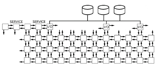
The Intel Paragon is a mesh connected, distributed memory multicomputer. It can have more than 1000 nodes connected in the form of a mesh. The Intel Paragon supports general purpose MIMD (Multiple Instruction Multiple Data) as well as the SPMD (Single Program Multiple Data) type of programming. Each node which consists of an i860 processor, has its own memory and its own copy of the operating system running on it to support the message passing protocols which are required to run a program on multiple processors. Each processor operates on its own data. Therefore to share data between the nodes, it requires message(s) to be sent from one node to the other. In this project, we have adopted the SPMD style of programming for our implementation. The NX message passing library for this purpose has been provided by Intel with the machine. The Paragon also supports other message passing protocols like PVM, P4 and tcmsg
As mentioned earlier, the SPMD style of programming was adopted in our approach. This style is well suited to our problem for the following reasons:
1. The operations being performed on each row of the data are the same if we consider the original projections row-wise (for each angle). Hence, the SPMD syle is well suited in the calculation of the filtered projections.
2. In the back projection stage, we have found that it can be implemented with very little message passing between the processors. For example, we need to send only as many messages as the number of processors for carrying out the entire back projection. This is a low overhead on the system. Care has been taken to ensure that the number of times a communication is requested is as low as possible (even if the size of the data being transmitted is large) to keep the total communication setup time to a minimum.
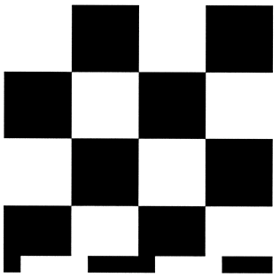
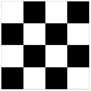
Since the serial algorithm carries out the FFT computations row-wise on each of the matrices P(n) and since the FFT operations on one row are independent from the other rows, it was decided to parallelize by distributing an equal number of rows to each processor. The projection data was generated by forward projecting a matrix of data which looked like a checker board. The size of the checker board was 16x16. The number of rows per processor was kept constant to support the SPMD style of programming. Since the data size was an integer multiple of 2, speed up results are available for 1,2,4,8 and 16 processors. Since the FFT algorithm works best for vectors which are integer powers of 2, zero padding has been done to keep the vector length of each row as an integer multiple of 2. Zero padding has the additional benefit of reducing the dishing and dc artifacts [3] inherent in the DFT algorithm. The FFT algorithm was run serially on all the processors, but each processor ran the algorithm on its own data. The maximum possible number of rays were used in all our simulations to project the data. For example, if the original data was a checker board of size 16x16, 16 rays were used to project the data and if the original data was 32x32, 32 rays were used. Increasing the number of rays beyond the number of pixels does not add any additional information as the value of density between these pixels is unknown. It must be noted that in the case of real objects, increasing the number of rays would lead to some extra information. Kak has mentioned that even in the case of real objects, increasing the number of rays beyond a reasonable limit does not lead to images which are any better [3].
Hence parallel computation of the filtered projections is done as follows:
1. Find Number of rows per processor = ( total number of rows ) / ( number of processors )
2. Initialize the H(n) and the projection matrix (PMAT) to zero to four times the number of rays. For example if the number of rays is 16, set the number of columns in H(n) and PMAT to 64. This basically takes care of the zero padding.
3. Evaluate H(n) on the 0th processor.
4. Pass the relevant rows to the various processors; e.g., if there are 16 processors being used with total number of rows=64, pass 4 rows to each processor with processor 0 having rows 1-4, processor 1 having rows 5-8, processor 2 having rows 9-12 and so on for all the 64 rows. (This matrix is called PMAT in the program).
5. Since the same response function is used all through, this data is passed on to all the processors by a single broadcast message from processor 0 to all other processors. The remaining operations are carried out in parallel.
6. On each processor, evaluate FFT for each of the rows of PMAT. That is, find the FFT of each row-vector row by row on each processor. This step proceeds in parallel on all processors. At the end of this, each row of PMAT contains its corresponding FFT sequence.
7. Multiply each element in each row of PMAT with the corresponding element from H (the response function). This step again proceeds in parallel on all the processors. The result of this operation is stored in the same matrix PMAT. Also, multiply each element of PMAT with a Hamming window function to reduce the Gibbs phenomenon. (Any other window function could also be used. Not multiplying with a Hamming window function would lead to more errors in the final image).
8. Evaluate the IFFT of PMAT row-wise. This is done in a standard way - find the complex conjugate of each row of PMAT and find its FFT. Then find its complex conjugate again and normalize. This step proceeds in parallel on all the processors.
This finds us the filtered projections.
Computation of the backprojections is as given by -

where x and y centroids, x_cen and y_cen respectively, represent the center along the x and y co-ordinate axes. Parallel implementation is carried out by splitting the above summation into smaller summations each of which can be computed in parallel. The results of these smaller summations are passed on to the zero'th processor which computes the total sum. The number of smaller summations into which the larger summation is split is equal to the number of processors, NP. The parallel algorithm (including the linear interpolation) is as follows:
For x = 1,x_max
For y = 1,y_max
For i = 1, rows / NP
1. Choose x, y and a theta_i.
2. Find t=((x-x_cen) / x_cen) cos(theta_i) + ((y-y_cen) / y_cen) sin(theta_i). Find the two points closest to the above and linearly interpolate between them to find Q(t) corresponding to the given x and y.
3, tmp_sum(x,y) = tmp_sum(x,y) + Q(t)
End for
End for
End for
4. Finally, Pass all the tmp_sum's to the zero'th processor to find the final sum.
The filtered back projection algorithm has been parallelized using the data parallel programming approach. The CM5 data network is well suited for data parallel programming as the machine has been designed for data parallel programming of large complex systems. The CM Fortran and C compilers support data parallel programming with a set of constructs [31] which allow users to program the machine for data parallelism. The CM5 runs the CMOST operating system which is based on UNIX with enhancements added to provide support for communication, time sharing and other activities important for running parallel programs. The user normally uses one of the high level programming languages provided on the machine (CM Fortran, C* or *LISP) which are derivatives of standard programming languages, but with parallel constructs to exploit the data parallel programming approach. The Connection Machine is made up of a large number of processors, each with its own local memory. While programming the CM5, emphasis is on the use of large uniform data structures, such as arrays whose elements can be processed at once. Depending on the size of the arrays, each element can be assigned to one processor or many elements can be assigned to one processor. The elements however remain distinct, and each element can be considered to have its own virtual processor [31]. Unless we specify otherwise, arrays of the same size and shape will have identical layouts, and a statement like A = B + C would proceed in parallel on all the elements with A having the same size as B and C. For interconnected data structures (like the FFT where a butterfly type of interconnection is required) the serial algorithm has to be modified suitably for running optimally on the CM5. For fastest execution, the entire algorithm may have to be modified to achieve maximum efficiency. Parallelism for finding the FFT has been accomplished by using the FFT routines available on the CM5 (in the CMSSL library) as they have already been optimized for this machine. It may be noted that even faster FFT algorithms have been tested on the CM5. Swartzrauber [32] has tested a parallel FFT on the CM5 which is claimed to be faster than the CMSSL FFT. However, to keep matters simple, the Connection Machine Scientific Subroutine Library (CMSSL) [33] has been used for finding the FFT's and Inverse FFT's.

We have taken the data parallel approach for which the CM5 has been designed. Since in the serial algorithm, the filtered projections are found row-wise on the projection data, it was decided to find the FFT row-wise serial, but parallel within each row by using parallel FFT provided by CMSSL. Evaluation of the Hamming function and multiplying the Fourier transformed projection data by the response function and the Hamming window function has also been done in parallel within each row, but serially row after row. Hence the algorithm for finding the filtered projections is:
For angle=1,K

	For col = 1,max_cols
	H2(col)=mat(angle,col) /* this assignment is also done in parallel for all elements in the row */
	End_for

	Find the FFT of H2 in parallel.

	Multiply H2 by the Hamming fn. and the filter fn.(ramp) in parallel.

	Find the IFFT of H2 in parallel.

	For col=1,max_cols
		mat(angle,col)=H2(col) /* done in parallel */
	End for
End for
This finds us the filtered projections.
The back-projection operation requires an efficient parallel implementation of interpolation. From the serial program, it can be seen that for each value of x,y and angle, a distinct value of t has to be evaluated. Also, the values of low-bin (lb), high-bin (hb) and the mid-bin (mb) are also distinct for different values of x,y and angle. Hence, to achieve parallelism t,lb,hb and mb have been made into 3D matrices. This enables the future operations using these matrices to be done in parallel by using the parallel constructs available on the CM5. The fractional values corresponding to the mid-bin's and the low-bin's are stored in frac which is also a 3D matrix. Since lb and hb are references to the columns of the 2D matrix containing the filtered projections (mat), a double referencing is made, and the values corresponding to the low-bin and high-bin are stored in 3D matrices (lbmat and hbmat). This allows us to carry out the linear interpolation in parallel (as is shown in the algorithm outlined below). Hence the parallel algorithm for back-projection is:
Each of the following steps is done in the order shown, but each step is executed in parallel:
For all x,y, and angle do in parallel each of the following steps:
1. Find t(x,y,angle)=((x-x_cen) / x_cen)* cos (theta) + ((y-y_{cen}/ y_{cen})* sin (theta)
2. Find mb(x,y,angle)=mp*t(x,y,angle)*correction + mp
3. Evaluate lb(x,y,angle) = truncate(mb(x,y,angle))
4. Evaluate frac(x,y,angle)=mb(x,y,angle)-lb(x,y,angle)
5. Evaluate hb(x,y,angle)=lb(x,y,angle)+1
6. Find lbmat(x,y,angle)=mat(angle,lb(x,y,angle))
7. Find hbmat(x,y,angle)=mat(angle,hb(x,y,angle))
8. For all x,y, and angle find the partial sums psum = lbmat + (hbmat-lbmat)*frac
Note the double referencing being done in the evaluation of lbmat and hbmat.
Finally, the densities can be found by summing over all the angles; this step is done in parallel by using the SUM function available on the CM5. This operation also proceeds in parallel; i.e.,
9. f(x,y) = sum of all the values of psum for all angles. This is done by summing the elements of psum over the angle (or third) dimension.
The simulations were performed for 1, 2, 4, 8 and 16 processors for the Intel Paragon and 32, 64, 128, 256 and 512 processors for the CM5. Plots of execution time, speed up and efficiency vrs. the number of processors have been made. The original images were of size 16x16, and the final images were 64x64 (due to zero padding). If the size of the original image is increased, then we can get better resolution in the final images. It should be noted that even though the final image is 64x64, it has information only from the original image which is 16x16.
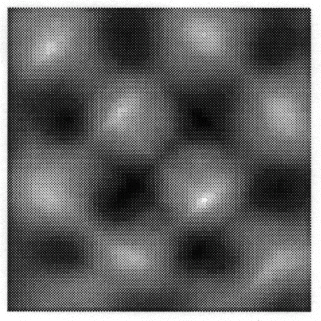
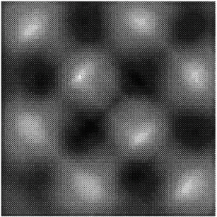
The execution times were averaged over 8 runs for each case and are tabulated below (Tables 4.1, 4.2, 4.3) It can be seen from the Matlab simulation results (Table 4.1) that most of the floating point operations are spent in evaluating the back-projections --- in fact the number of floating point operations for back-projections exceed those of the filtered projections by more than 14 times. Most of the cpu-time is therefore spent in evaluating the back-projections in both the parallel and the serial programs. Most of the speed up in the parallel programs is a result of the parallelization of the back-projections. Figures 4.1 and 4.2 show the original and the reconstructed images for the Paragon and figures 4.6 and 4.7 show the same for the Connection Machine (CM5). Figures 4.3, 4.4 and 4.5 show the trends in the execution time, speedup and efficiency for the Paragon. Figures 4.8, 4.9, 4.10 and 4.11 show the speedup and efficiency trends in the case of the Connection Machine (CM5).
Speed up and efficiency has been calculated in the following manner:


For the block efficiency curve of the CM5 in fig. 4.11 the following formula has been used:

That is, the efficiencies have been normalized with respect to the efficiency of 32 processors on the CM5. This has been done because the minimum partition on the CM5 is a 32 node partition, and the other partitions must be a power of 2. Table 4.1 shows the simulation of the algorithm using Matlab on a Sun Sparc 10. It can be seen that the most of the floating point operations are consumed in the back-projection stage (about 93% of the total). Tables 4.2 and 4.3 show the simulations done on the Intel Paragon and CM5 respectively. The number of Million Floating Point Operations Per Second (MFLOPS) has been found by dividing the total number of floating point operations by the total time. It can be seen that the best simulation times are obtained with 8 processors on the Paragon and 256 processors on the CM5. Overall the Paragon seems to offer a better performance in terms of efficiency. Some preliminary simulations on the breakup of execution times between filtered projections and backprojections show that the CM5 takes longer for the filtered projections, and the Paragon takes longer for the backprojections. The times for the filtered projections on the Paragon show a variation of as much as 40% in the 4 processor case. In the other cases, the variation was about 20% maximum. All the times shown here have been averaged over several runs (8 to 10) to get representative times for each case. On the CM5, the consistency was better and the times were consistent to about 10%.
It can be seen from the simulation results that in the case of CM5 the execution time is consistently dominated by the filtered projections, whereas in the case of the Paragon, the execution time is dominated by the back-projections.


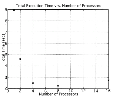
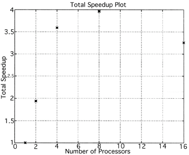
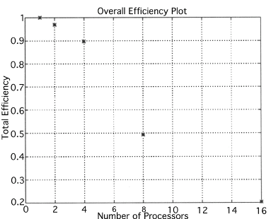
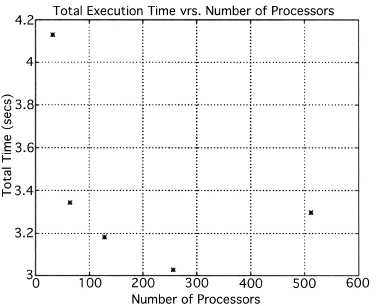
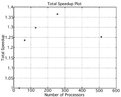
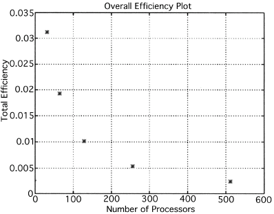
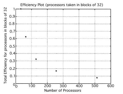
The Filtered Backprojection Algorithm has been parallelized and run on a multiprocessor Intel Paragon and Connection Machine CM5. The algorithm has been analyzed for efficiency and speedup on both the Intel Paragon and the CM5. It was observed that maximum speedup is about 4 for the Intel Paragon and 1.36 for the CM5 (CM5 speedups are with respect to the 32 processor times). Overall, the results on the Intel Paragon (speed-up and efficiency) seem to be better than on the CM5. This could be due to the greater communication requirements between the processors of the CM5 as compared to the Intel Paragon. The larger number of processors on the CM5 also adds to the communication overhead. The maximum speed-up occurs for 8 processors on the Intel Paragon, and for 256 processors on the CM5. Speedup has been achieved mainly due to the parallelization of the back-projections, as most of the floating point operations are consumed in the back projection stage in the serial code. On the Paragon, in the back-projection stage, the splitting of the summation among different processors cannot be done indefinitely. At some point, the time taken to compute the partial summations will be less than the time for passing the results to the zeroth processor. At this point, increasing the number of processors will increase the execution time. On the CM5 the large memory requirements may be a disadvantage. The execution times obtained from the parallelization on the two machines indicate that at least in the 2D case real time performance can be expected.
From the simulations, it is seen that the CM5 algorithm spends most of the time on calculating the filtered projections, and the Paragon in the calculating the back-projections. This difference in the two machines is primarily due to differences in the implementation.
 Return to Visualization Home Page
http://www.sv.vt.edu/xray_ct/parallel/Parallel_CT.html
Revised April 5, 1995