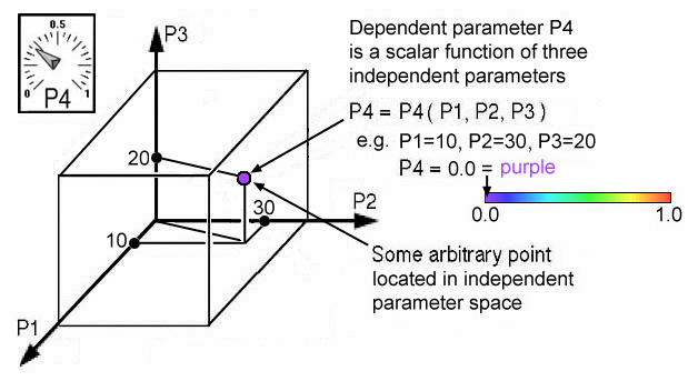
Figure 18. Four parameter space
Unlike Fig. 3 the scalar function notation P4(P1,P2,P3) is used instead of f(x,y,z) which emphasizes the use of "P" for both dependent and independent parameters. Hence the function shown in Fig. 18 is referred to as a four parameter space. For example the following scalar function P4=f(x,y,z) defines the surface, S, of the spherical function with it's center located at P1=x=10, P2=y=30, and P3=z=20. Both functional forms are shown below for comparison. Either function locates the origin of the sphere, such that P4=S=0.0, which is shown as a purple point in Fig. 18.
     S = f(x,y,z)     = (x-10)2 + (y-30)2 + (z-20)2                 (4)
    P4 = P4(P1,P2,P3) = (P1-10)2 + (P2-30)2 + (P3-20)2              (5)
If three orthogonal planes intersect at the point shown in Fig. 18, concentric
circular color gradients would be seen in each plane. However isosurface plots
could also be used to show concentric spheres. If an interactive dial for P4
is increased from 0.0 the isosurface would increase in size and contract in
size when P4 is decreased. This expanding-contracting isosurface in the
neighborhood of a point is our simplest idea of a 3D gradient. Isosurfaces,
can show only one ("iso") value for parameter P4 which is drawn as a surface
connecting all of the same values for P4 in parameter space. Surfaces in
general may not be continuously connected. The example here is a continuous
function which generates a single smooth continuous spherical surface.
Isosurfaces are typically drawn as Gouraud shaded surfaces that emphasize
surface irregularities that correspond to small gradient changes. Hence
isosurfaces work best for irregular shaped functions.
From our experience from experiments and analysis we expect to find irregular isosurfaces when envisioning how a property is distributed in space (x,y,z). Here we show results from a numerical simulation of gas mixing with air, Brown [7]. An isosurface of 50% gas concentration is shown in Fig. 19.
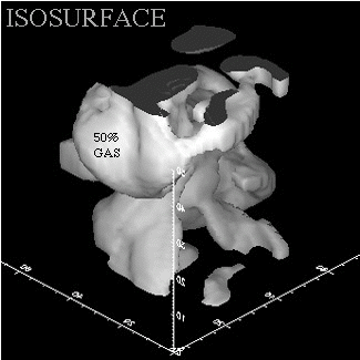
Figure 19. Volume visualization of gas mixing with air. Numerical simulation on the CM-2 computer at Naval Research Labs, Brown [7].
An isosurfaces shows only one value of gas concentration, but voxel volume translucency, used in Fig. 20, shows all values of gas concentration ranging from 0% (transparent) to 100% (white-opaque) over the entire volume. However the gradient in P4 (gas concentration) can only be seen if this volume gradient is rotated. Click on the image in Fig. 20 to generate this rotation animation.
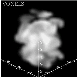
Figure 20. Voxels reveals the gradation of a gas-air mixture over the entire volume, where 0% gas concentration is rendered transparent and 100% gas concentration is rendered white-opaque. The 3D gradient in gas concentration is only revealed if rotated. Generate rotational animation by clicking on image.
This ability to see 3D gradients of a scalar function, P4, in parametric space is an excellent example of our inherent cognitive abilities to reconstruct 3D volumes from 2D images. Note that each image in this animation contains only 2D gradients. The human mind can reconstruct volumetric 3D information from 2D images much the same as computer tomography reconstruction. Whereas fast computers are required to reconstruct these 3D gradients, the human mind does this instantaneously. So how is this possible? The human mind invokes the same simple idea used in all computer reconstruction algorithms -- backprojection.
Backprojection as the name implies projects a sequence of 2D image gradients back into a 3D volume. Imagine creating an ordered sequence of 2D X-Ray images of a human head by rotating the human head shown in Fig. 21. Each 2D image, shown in Fig. 22 is a projection of X-Ray density onto a 2D plane. Backprojection is simply reversing this process.
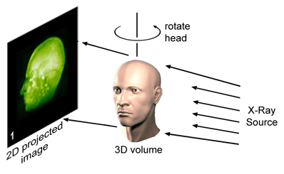
Figure 21. Schematic of creating a sequence of 2D X-Ray images of a rotating human head
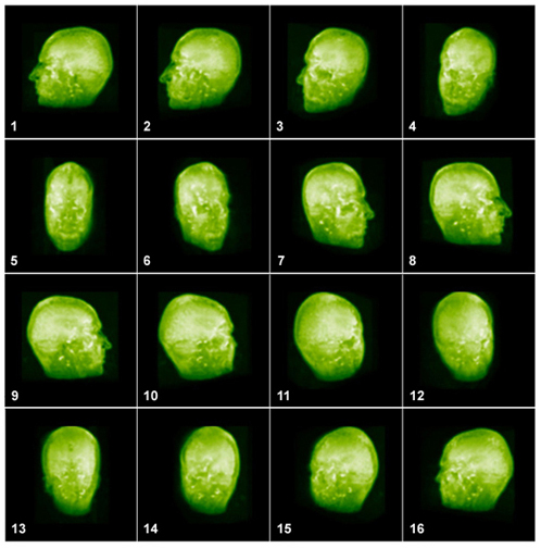
Figure 22. Sequence of 2D X-Ray images of a rotating human head shown as as a small multiple. Animation of this ordered 2D image sequence reconstructs the head into a 3D volume. Generate rotation animation by Clicking on image.
Imagine that the images shown in Fig. 22 are layed out on the inside surface of a circular cylinder in the same sequence they were generated. If each of these images are projected back into the center of the cylinder a volumetric 3D image can be reconstructed. When the same ordered seqence of 2D X-Ray images of the human head is viewed as an animation, the human eye and mind reconstructs the 3D volume and 3D gradients are preceived. In a sense this human perception is a cognitive implementation of back projection. This same technique was used to view 3D gradients of gas concentration in Fig. 20. It is also possible to view 4D gradients of gas concentrations by showing how 3D volume gradients change with a corresponding change in time, the fourth dimension. This is possible if the change in 3D volume gradients at each time increment is shown for each corresponding rotational increment in the animation. Other independent parameters could be selected instead of time. However this technique is limited to four independent variables. Again it is important to remember that independent parameter space is not limited to rectangular cartesian coordinates.
Often there is more than one scalar function. For example, pressure and temperature can simultaneously exist within the same region where parameters along the axes become x, y, and z coordinate space. From our previous method it is not possible to view gradients of more than one scalar function at the same time, simply because we can see only one color. However multiple scalar functions can be observed in the same parametric space where the viewer can test for the existence of new relationships between these functions.
This visual method is developed in terms of multiple parameters, which are defined either as m-independent or n-dependent parameters. The example shown in Fig.23 is a seven parameter model. The first three parameters (P1, P2, P3) are independent variables, shown here as orthogonal axes, and the fourth orthogonal parameter is reserved as another independent variable that exists uniformly the same everywhere, but which can not be drawn as an axis: i.e. P4 = time (the fourth orthogonal axis that can not be shown). It is important to note that in Fig. 18, P4 is a dependent parameter and in Fig. 23, P4 is an independent parameter. Because the three dependent parameters (P5,P6,P7) are scalar functions that share the same independent parametric space, only three of which can be seen, this method provides a common basis from which to test for the existence of relationships between these three functions. In the development of this method it is important to note the difference between the dependent parameters (P5,P6,P7), which are functions of independent parameters (P1,P2,P3,P4), and the functional relationship between the P5, P6, and P7 functions. Our goal is to determine this functional relationship.
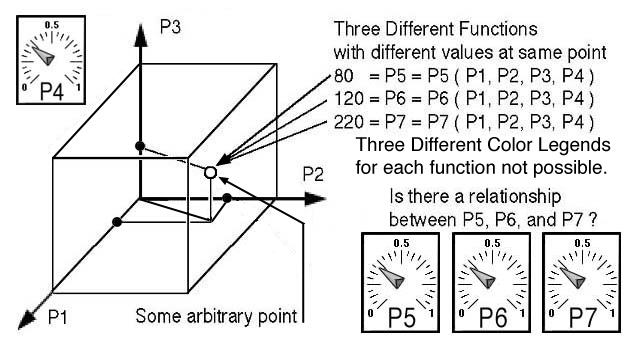
The visual task is to find the functional relationship between P5, P6, and P7, if any exists. The key idea here is that not all independent parameters have to be visually represented as coordinates, but can be varied independently by using an interactive graphical interface such as the moving dial for P4 shown in Fig.23.
At some arbitrary point in Fig. 23 each scalar function has a unique value: e.g. P5 = 80, P6 = 120, and P7 = 220. Units are intentionally not shown. Obviously these values can change at adjacent points. This is our idea of a gradient. Although it is not possible to see all possible values for all three functions in the same region, it is possible to see an isosurface for each function as a separate shaded surface that intersect at a common but arbitrary point. If the observer can interactively change the isosurface value in Fig. 23 and instantaneously observe the corresponding change in shape of the intersecting isosurface, then a gradient near this point could be determined for each function, but only in that immediate region. For example, if the scalar property were fluid pressure it would be possible to envision the flow direction.
Although it is highly recommended to think of the physics as a visual method is used to analyze a data set, it is important that the visual method first be developed only with respect to the property of mathematical invariance. Consequently this visual method can be used for any arbitrary set of scalar functions (dependent parameters) that share a common set of independent parameters. For this reason a 3D data set without units is presented where two of the three dependent parameters are drawn as unique but intersecting isosurfaces in Fig. 24. If the surfaces do not intersect then it is not possible to determine a functional relationship between P5, P6, and P7. If the surfaces intersect, then there is an opportunity to investigate if this functional relationship is linearly proportional or inversely proportional.
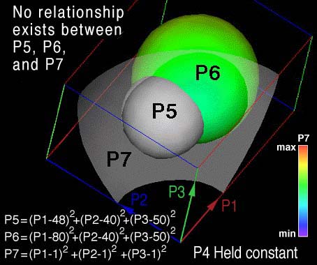
Figure 24. No relationship exists between P5, P6, and P7.
It is not necessary to determine the functional form of each dependent parameter P5, P6, and P7 by a curve fitting method. In fact the functional relationship between P5, P6, and P7 can be determined without knowing anything about the dependent parameter functions. Many data sets are generated by experimental scanning or numerical simulations and lack a functional form to begin with. Curve fitting these dependent parameter functions is avoided and our attention focuses on how these arbitrary shapes (arbitrary functions) relate only to each other. If the three dependent parameters are arbitrarily chosen as spherical functions, then P5 and P6 can be conveniently viewed as nonconcentric intersecting spheres in Fig. 24.
This visual method tests for functional relationships between P5, P6, and P7. The method assumes P7 is just another dependent parameter that may or may not be related to P5 or P6. A possible functional relationship is confirmed when P7 is mapped as a color onto the P6 isosurface and color gradients would be seen to align with the P5-P6 intersection in Fig. 24. Because of the small range of colors for P7, the alignment of P7 color gradients is difficult to see on the P6 isosurface (mostly green) therefore P7 is also represented as an isosurface in Fig. 24. Alignment of the P7 color or isosurface at P5-P6 intersection is not observed which visually demonstrates that there can be no functional relationship between P5, P6, and P7 in Fig. 24. However, if P7 is observed as a constant color near the P5-P6 intersection as shown in Fig. 25 or if the P7 isosurface intersection occurs near the P5-P6 intersection, then a simple linear functional relationship exists between P5, P6, and P7. In both Fig. 24 and Fig. 25 the independent parameter P4 is held constant.
Results shown in Fig. 25 only confirm that simple linear relationships exist, which could be one of three possible relationships:
              P5 P6 P7  = constant,                   (6)
              P5 P6 = constant P7,                    (7)
              P5 = constant P6 P7.                    (8)
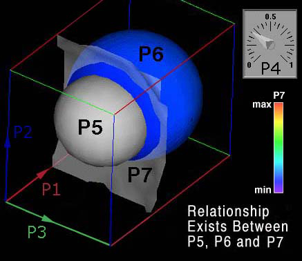
Figure 25: Simple proportional and inversely proportional relationships exist for P5, P6, and P7. P7 is rendered as a translucent isosurface, so that the observer can better view the small changes in color for the P7 property.
These equations will be eliminated or confirmed visually in Fig. 25. If P6 is held fixed while the P5 isosurface is arbitrarily increased and the color or surface for P7 is observed to increase near the P5-P6 intersection, then Eqn. (6) is eliminated as a possible functional relationship. If P5 is held fixed while the P6 isosurface is arbitrarily increased and the color or surface for P7 is observed to decrease near the P5-P6 intersection, then Eqn. (7) is also eliminated as a possible functional relationship, but Eqn. (8) is satisfied where P4 was held constant. Finally, if parameters P5, P6, and P7 are all held fixed and only P4 is changed and if similar intersecting patterns are observed at any arbitrary value for P4, then the surviving functional relationship, Eqn. (8), is valid over the entire parametric space P1, P2, P3, and P4. Again it is important to note the functional shape of P5, P6, and P7 are arbitrary and independent of the process that confirms the existence of functional relationships between P5, P6, and P7.
Here the mathematical idea of arbitrariness and invariance was used to visually confirm the existence of a scalar tensor equation for arbitrary variations in dependent parameters P5, P6, and P7. In this example there are two different types of mathematical invariance. For Eqn. (8) we have a simple zeroth order tensor equation where not only are the scalar dependent parameters P5, P6, and P7 invariant to arbitrary RCC transformations at a point, but the same scalar equation itself is also invariant to any arbitrary variation that exists through out parametric space, P1, P2, P3, and P4. Both types of mathematical invariance are related to our idea of a physical law: that is, the parameters P5, P6, and P7 must always satisfy the same functional relationship independent of any arbitrary change that exists within parametric space P1, P2, P3, and P4. This same visual-mathematical paradigm of invariance can be extended to higher order tensor equations.
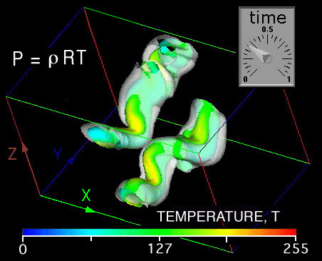
Figure 26. Extracting a linear zeroth order tensor equation from numerical data of a simulation where mixing occurs in a boundary layer at supersonic speeds, Ragab [8]. Temperature is intentionally left nondimensional.
Simple scalar relationships, such as Eqn. (8), commonly occur in nature. For example let P1, P2, P3 be RCC coordinate space and P4 is time, and let P5, P6, and P7 be pressure, P, density, ρ, and temperature, T, respectively in Fig. 26 and the constant in Eqn. (8) becomes the gas constant, R, in Eqn. (9), which is the gas law.
P = ρ R T (9)
This visual interactive function extraction method would be particularly useful in an immersive environment where with head tracking the observer could verify intersecting isosurface color maps by penetrating isosurfaces anywhere within RCC space that are obscuring the observer's view.
Closing Comments on Extracting Simple Linear Algebraic Expressions from a Uniform Distribution of Numbers in Compressed Parametric Space
We have been successful in finding many more complex functions using this same method. But because of space we have provided only an example of a simple linear relationship. In all cases, just like finding solutions to differential equations, we must guess at possible solutions. This guess can then be visually confirmed by constructing the necessary visual computer program modules that provide unique features required for the visual confirmation. This same idea is used when approximating functions using a Taylor series, where the first term in the series are simple linear terms. Higher ordered terms in the series can be included, but for a first approxiation it is common practice to investigate the linear terms. Within the cognitive visual data compression (CVDC) format the researcher can explore large complex data sets for trends and possible functions. Because our visual format requires uniformly distributed numbers, this method can be used with experimental data as well as numerical solutions. First a pattern of scalar functions is drawn than thought becomes the cognitive mechanism that allows the investigator to confirm the existence of functional relationships embedded in these scalar functions. Again we use the computer to perform tedious tasks where in the past only a few gifted scientists demonstrated an inherent ability to perform this same task psychically.
Original: http://www.sv.vt.edu/classes/ESM4714/methods/FuncExt.html
Current: http://www.sv.rkriz.net/classes/ESM4714/methods/FuncExt.html