Sources of Scientific Data Sets
The most common source of data comes from numerical simulations where we predict gradients in physical properties both in space and time. If properly organized the viewer can begin to interpret not only the large volume of data but also to understand how property relationships change in space and time.
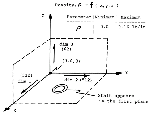
Perhaps the best known 3-D experimental data source is the X-ray computed tomography (CT) scan where we observe gradients in density. Instead of the more common biomedical application, here we introduce a material application where the source of data is a CT scan of a turbine fan blade. The objective is visual detection of the existence, location and 3-D distribution of cracks, voids, or other inhomogeneities which are physically significant. Below we show how these data are organized.

Figure 1. Schematic of Density Distribution Measured by X-rays with a Computer Tomography (CT) Scan System.
You can get more information about how this data set is organized on your optical disk, along with PV-Wave procedure files that will be used to visualize the data.
You can also get some background information, Problem Statement and Visual Insight, about this data set from the researcher who worked this data set.
Typical CT scanners can measure 512 slices parallel to the x-y plane where each slice contains 512 x 512 individual measurements points. The final result is a volume of 134,217,000 points. If each point (a volume of 20 x 20 x 20 um) is represented by 256 shades of gray or 256 colors then we require 8 bits of memory for each data point which will total 1 gigabits of memory for a complete scan. Obviously 3-D graphical tools can help us sort through this large data set.
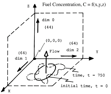
Figure 2. Parameters Defined for Gas-Air Elliptic Jet Mixing Simulation
Example of how this ASCII data set was created and organized into 3-D format.
       program name
       integer image(64,64,44)
       open(6,file='brown.ascii.start',status='unknown',err=888)

            --  numerical calculations for fuel concentrations  --

            --  Scale concentration into integers  ( 0 min.  to  255 max )  --

       write(6,10)(((image(i,j,k),i=1,64),j=1,64),k=1,44)
    10 format(64(1x,i3))
    88 stop
       end
You can view the FORTRAN program used
to create a SDS-HDF file of this data set.
You can get more information about how this data set is organized on your optical disk, along with PV-Wave procedure files that will be used to visualize the data.
You can also get some background information, Problem Statement and Visual Insight, about this data set from the researcher who worked this data set.
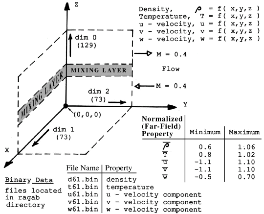
Three dimensional graphical tools can also be used to study how distributed properties are
interrelated in space and change with time. Below is a numerical simulation of two volumes
mixing along a common interface where the relationships of density, temperature, and the
u,v,w velocity components can be observed to change with time.
Figure 3. Parameters Defined for a Compressible Mixing Layer.
For Assignment#3 you will need to know how this binary data was normalized and scaled
You can get more information about how this data set
is organized on your optical disk, along with PV-Wave procedure files that will be used
to visualize the data.
You can also get some background information, Problem
Statement and Visual Insight, about this data set from the researcher who worked this data
set.
The advantages of using these 3-D graphic tools in coordinate space can be extended to
parameter space. Again the source of data sets for parameter space can be from
experimental, analytical, or numerical origins. The idea is the same, that is, to use the same
3-D visual tools we used in coordinate space to help in our visual thinking (analysis) of how
properties are related to other parameters where these other parameters are substituted for the
x,y,z coordinate axes, hence the name "parameter space". Parameter space visualization is
only for those who are intimately involved with their data sets and require yet another
dimension for interpretation and evaluation.
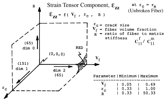
An excellent example is given below where we can observe the relationship of strain
concentration at a fiber/matrix interface as a function of an approaching crack, surrounding
fiber volume fraction, and the ratio of the fiber/matrix moduli. The objective here is to use
the visual tools to better understand how these four properties (parameters) are related.
ANALYTICAL (parameter space): One property: strain concentration.
Figure 4. Parameters Defined for Composite Material Fracture Model where
the Axial Strain in the Unbroken Fibers are Plotted as a Function of Crack Length,
Fiber Volume Fraction, and Ratio of Fiber to Matrix Modulus.
You can get more information about how this
data set is organized on your optical disk, along with PV-Wave procedure files
that will be used to visualize the data.
You can also get some
background information, Problem Statement and Visual Insight, about this data set from
the researcher who worked this data set.
Because parameter space is often unique to the observer-researcher we will not elaborate on
this example although 3-D parameter viewing of data has the most opportunity for visual
discovery.
Next, let us see how researchers have used visual tools with these different data sources to
gain an understanding of the physically significant relationships embedded in their data.
http://www.sv.vt.edu/classes/ESM4714/data_sets/data_sets.html
NUMERICAL (coordinate space): Five properties: Density, temperature, and u,v, and w
velocities
3. Parameter Space
End of Information on Sources of Scientific Data Sets
 Return to Visualization Home Page
Send comments to: rkriz@vt.edu
Ronald D. Kriz
Virginia Tech
College of Engineering
Revised April 4, 1995